UPDATED: 5/20/2021

A version of this post was originally published over at Conversion XL

For all of the talk about how awesome (and big, don’t forget big) Big data is, one of the favorite tools in the conversion optimization toolkit, AB Testing, is decidedly small data. Optimization, winners and losers, Lean this that or the other thing, at the end of the day, A/B Testing is really just an application of sampling.

You take couple of alternative options (eg. ‘50% off’ v ‘Buy One Get One Free’ ) and try them out with a portion of your users.  You see how well each one did, and then make a decision about which one you think will give you the most return.  Sounds simple, and in a way it is, yet there seem to be lots of questions around significance testing. In particular what the heck the p-value is, and how to interpret it to help best make sound business decisions.

These are actually deep questions, and in order to begin to get a handle on them, we will need to have a basic grasp of sampling.

A few preliminaries

Before we get going, we should quickly go over the basic building blocks of AB Testing. I am sure you know most of this stuff already, but can’t hurt to make sure everyone is on the same page:

The Mean – often informally called the average. This is a measure of the center of the data. It is a useful descriptor, and predictor, of the data, if the data under consideration tends to clump near the mean AND if the data has some symmetry to it.

The Variance – This can be thought of as the average variability of our data around the mean (center) of the data.  For example, consider we collect two data sets with five observations each: {3,3,3,3,3} and {1,2,3,4,5}.  They both have the same mean (its 3) but the first group has no variability, whereas the second group does take different values than its mean. The variance is a way to quantify just how much variability we have in our data.  The main take away is that the higher the variability, the less precise the mean will be as a predictor of any individual data point.

The Probability Distribution – this is a function (if you don’t like ‘function’, just think of it as a rule) that assigns a probability to a result or outcome.  For example, the roll of a standard die follows a uniform distribution, since each outcome is assigned an equal probability of occurring (all the numbers have a 1 in 6 chance of coming up).  In our discussion of sampling, we will make heavy use of the normal distribution, which has the familiar bell shape.  Remember that the probability of the entire distribution sums to 1 (or 100%).

The Test Statistic or Yet Another KPI
The test statistic is the value that we use in our statistical tests to compare the results of our two (or more) options, our ‘A’ and ‘B’.   It might make it easier to just think of the test statistic as just another KPI.  If our test KPI is close to zero, then we don’t have much evidence to show that the two options are really that different. However, the further from zero our KPI is, the more evidence we have that the two options are not really performing the same.

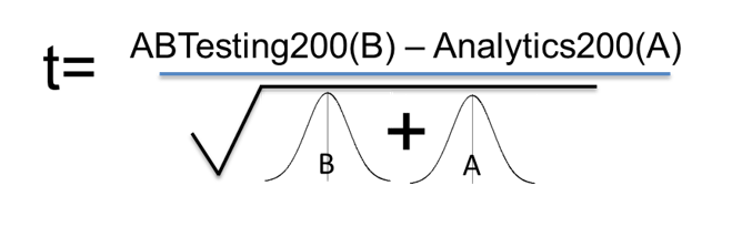
Our new KPI combines both the differences in the averages of our test options, and incorporates the variability in our test results. The test statistics looks something like this:

While it might look complicated, don’t get too hung up on the math. All it is saying is take the difference between ‘A’ and ‘B’ – just like you normally would when comparing two objects, but then shrink that difference by how much variability (uncertainty) there is in the data.

So, for example, say I have two cups of coffee, and I want to know which one is hotter and by how much. First, I would measure the temperature of each coffee. Next, I would see which one has the highest temp. Finally, I would subtract the lower temp coffee from the higher to get the difference in temperature. Obvious and super simple.

Now, let’s say you want to ask, “which place in my town has the hotter coffee, McDonald’s or Starbucks?” Well, each place makes lots of cups of coffee, so I am going to have to compare a collection of cups of coffee. Any time we have to measure and compare collections of things, we need to use our test statistics.

The more variability in the temperature of coffee at each restaurant, the more we weigh down the observed difference to account for our uncertainty. So, even if we have a pretty sizable difference on top, if we have lots of variability on the bottom, our test statistic will still be close to zero. As a result of this, the more variability in our data, the greater an observed difference we will need to get a high score on our test KPI.

Remember, high test KPI -> more evidence that any difference isn’t just by chance.

Always Sample before you Buy

Okay now that we have that out of the way, we can spend a bit of time on sampling in order to shed some light on the mysterious P-Value.

For sake of illustration, let say we are trying to promote a conference that specializes in Web analytics and Conversion optimization.  Since our conference will be a success only if we have at least certain minimum of attendees, we want to incent users to buy their tickets early. In the past, we have used ‘Analytics200’ as our early bird promotional discount code to reduce the conference price by $200.  However, given that AB Testing is such a hot topic right now, maybe if we use ‘ABTesting200’ as our promo code, we might get even more folks to sign up early. So we plan on running an AB test between our control, ‘Analytics200’ and our alternative ‘ABTesting200’.

We often talk about AB Testing as one activity or task. However, there are really two main parts of the actual mechanics of testing.

Data Collection – this is the part where we expose users to either ‘Analytics200’ or ‘ABTesting200’. As we will see, there is going to be a tradeoff between more information (less variability) and cost.  Why cost? Because we are investing time and foregoing potentially better options, in the hopes that we will find something better than what we are currently doing. We spend resources now in order to improve our estimates of the set of possible actions that we might take in the future. AB Testing, in of itself, is not optimization. It is an investment in information.

Data Analysis – this is where we select a method, or framework, for drawing conclusions from the data we have collected. For most folks running AB Tests online, it will be the classic null significance testing approach. This is the part where we pick statistical significance, calculate the p-values and draw our conclusions.

The Indirect logic of Significance Testing

Toni and Nate are waiting for the subway.  Toni is a local and takes the subway almost every night.  This is Nate’s first time in the city and has never taken the subway before. Nate asks Toni about how long it normally takes for the train to come.  Toni tells him that usually she waits about five minutes.  After about 15 minutes of waiting, Nate starts to get worried and thinks maybe there is a problem with the train and perhaps they should just go and try to catch a cab instead.  He asks Toni, ‘Hey, I am getting worried the train might not come. You said the train takes about five minutes on average, how often do you have to wait 15 minutes or more?’  Toni, replies, ‘don’t worry, while it usually comes in about five minutes, it is not uncommon to have wait this long or even a bit longer. I’d say based on experience, a wait like this, or worse, even when there is no issue with the subway, probably happens about 15% of the time.’ Nate relaxes a bit, and they chat about the day while they wait for the train.

Notice that Nate only asked about the frequency of long wait times.  Once he heard that a wait time of 15 min or more wasn’t too uncommon even when the trains are running normally, he felt more comfortable that the train was going to show up.  What is interesting is what he learns is NOT the probability that trains aren’t working.   Rather he learns, based on all the times that Toni has taken the train, the probability of the train running late more than 15 minutes when there are no service issues.  He concludes that the train is likely working fine since his wait time isn’t too uncommon, NOT because he knows the probability that the train has an issue. This indirect, almost contrarian logic is the essence of  hypothesis testing. The P-Value in this case is the probability that the wait times are 15 min or more given that the trains are running normally.

Back to our Conference

For the sake of argument, let’s say that the ‘Analytics200’ promotion has a true conversion rate of 0.1, or 10%.  In the real world, this true rate is hidden from us – which is why we go and collect samples in the first place –  but in our simulation we know it is 0.1. So each time we send out ‘Analytics200’, approximately 10% sign up.

If we go out and offer 50 prospects our ‘Analytics200’ promotion we would expect, on average, to have 5 conference signups. However, we wouldn’t really be that surprised if we saw a few less or a few more.  But what is a few? Would we be surprised if we saw 4? What about 10, or 25, or zero?   It turns out that the P-Value answers the question, How surprising is this result?

Extending this idea, rather than taking just one sample of 50 conference prospects, we take 100 separate samples of 50 prospects (so a total of 5,000 prospects, but selected in 100 buckets of 50 prospects each).  After running this simulation, I plotted the results of the 100 samples (this plot is called a histogram) below:

Our simulated results ranged from 2% to 20% and the average conversion rate of our 100 samples was 10.1% – which is remarkably close to the true conversion rate of 10%.

Amazing Sampling Fact Number 1

The mean (average) of repeated samples will equal the mean of the population we are sampling from.

Amazing Sampling Fact Number 2

Our sample conversion rates will be distributed roughly according to a normal distribution – this means most of the samples will be clustered around the true mean, and samples far from our mean will occur very infrequently.  In fact, because we know that our samples are distributed roughly normally, we can use the properties of the normal (or students-t) distribution to tell us how surprising a given result is.

This is important, because while our sample conversion rate may not be exactly the true conversion rate, it is more likely to be closer to the true rate than not.  In our simulated results, 53% of our samples were between 7 and 13%. This spread in our sample results is known as the sampling error.

Ah, now we are cooking, but what about sample size you may be asking? We already have all of this sampling goodness and we haven’t even talked about the size of each of our individual samples. So let’s talk:

There are two components that will determine how much sampling error we are going to have:

• The natural variability already in our population (different coffee temperatures at each Starbucks or McDonald’s)
• The size of our samples

We have no control over variability of the population, it is what it is.

However, we can control our sample size. By increasing the sample size we reduce the error and hence can have greater confidence that our sample result is going to be close to the true mean.

Amazing Sampling Fact Number 3

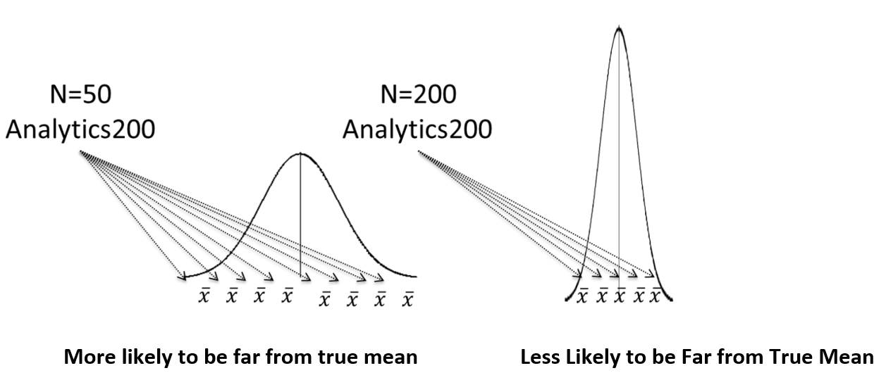
The spread of our samples decreases as we increase the ‘N’ of each sample.  The larger the sample size, the more our samples will be squished together around the true mean.

For example, if we collect another set of simulated samples, but this time increase the sample size to 200 from 50, the results are now less spread out – with a range of 5% to 16.5%, rather than from 2% to 20%. Also, notice that 84% of our samples are between 7% and 13% vs just 53% when our samples only included 50 prospects.

We can think of the sample size as a sort of control knob that we can turn to increase or decrease the precision of our estimates.  If we were to take an infinite number of our samples we would get the smooth normal curves below. Each centered on the true mean, but with a width (variance) that is determined by the size of each sample.

Why Data doesn’t always need to be BIG

Economics often takes a beating for not being a real science, and maybe it isn’t ;-). However, it does make at least a few useful statements about the world. One of them is that we should expect, all else equal, that each successive input will have less value than the preceding one. This principle of diminishing marginal returns is at play in our AB Tests.

Reading right to left, as we increase the size of our sample, our sampling error falls. However, it falls at a decreasing rate – which means that we get less and less information from each addition to our sample.   So in this particular case, moving to a sample size of 50 drastically reduces our uncertainty, but moving from 150 to 200, decreases our uncertainty by much less. Stated another way, we face increasing costs for any additional precision of our results. This notion of the marginal value of data is an important one to keep in mind when thinking about your tests. It is why it is more costly and time consuming to establish differences between test options that have very similar conversion rates.  The hardest decisions to make are often the ones that make the least difference.

Our test statistic, which as noted earlier, accounts for both how much difference we see between our results and for how much variably (uncertainty) we have in our data. As the observed difference goes up, our test statistic goes up. However, as the total variance goes up, our test statistic goes down.

Now, without getting into more of the nitty gritty, we can think of our test statistic essentially the same way we did when we drew samples for our means.  So whereas before, we were looking just at one mean, now we are looking at the difference of two means, B and A.  It turns out that our three amazing sampling facts apply to differences of means as well.

Whew- okay, I know that might seem like TMI, but now that we have covered the basics, we can finally tackle the p-values.

Assume There is No Difference

Here is how it works. We collect our data for both the ABTesting200, and Analytics200 promotions. But then we pretend that really we ran an A/A test, rather than an A/B test. So we look at the result as if we just presented everyone with the Analytics200 promotion.  Because of what we now know about sampling, we know that both groups should be centered on the same mean, and have the same variance – remember we are pretending that both samples are really from the same population (the Analytics200 population). Since we are interested in the difference, we expect that on average, that Analytics200-Analytics200 will be ‘0’, since on average they should have the same mean.

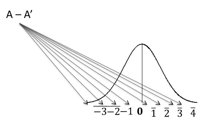
So using our three facts of sampling we can construct how the imagined A/A Test will be distributed, and we expect that our A/A test, will on average, show no difference between each sample. However, because of the sampling error, we aren’t that surprised when we see values that are near zero, but not quite zero. Again, how surprised we are by the result is determined by how far away from zero our result is. We will use the fact that our data is normally distributed to tell us exactly how probable seeing a result away from zero is. Something way to the right of zero, like at point 3 or greater will have a low probability of occurring.

Contrarians and the P-Value, Finally!

The final step is to see where our test statistic falls on this distribution. For many researchers, if it is somewhere between -2 and 2, then that wouldn’t be too surprising to see if we were running an A/A test. However, if we see something on either side of or -2 and 2 then we start getting into fairly infrequent results. One thing to note: what is ‘surprising’ is determined by you, the person running the test.  There is no free lunch, at the end of the day, your judgement is still an integral part of the testing process.

Now lets  place our test statistic (t-score, or z-score etc) on the A/A Test distribution. We can then see how far away it is from zero, and compare it to the probability of seeing that result if we ran an A/A Test .

Here our test statistic is in the surprising region.  The probability of the surprise region is the P-value. Formally, the p-value is the probability of seeing a particular result (or greater) from zero, assuming that the null hypothesis is TRUE.  If ‘null hypothesis is true’ is tricking you up, just think instead, ‘assuming we had really run an A/A Test.

If our test statistic is in the surprise region, we reject the Null (reject that it was really  an A/A test). If the result is within the Not Surprising area, then we Fail to Reject the null.  That’s it.

Conclusion: 7 Points

Here are a few important points about p-values that you should keep in mind:

• What is ‘Surprising’ is determined by the person running the test. So in a real sense, the conclusion of the test will depend on who is running the test.  How often you are surprised is a function of how high a p-value you need to see (or related, the confidence level in a Pearson-Neyman approach, eg. 95%) for when you will be ‘surprised’.
• The logic behind the use of the p-value is a bit convoluted. We need to assume that the null is true in order to evaluate the evidence that might suggest that we should reject the null. This is an evergreen source of confusion.
• It is not the case that the p-value tells us the probability that B is better than A. Nor is it telling us the probability that we will make a mistake in selecting B over A. These are both extraordinarily commons misconceptions, but they are false.  This is an error that even ‘experts’ often make, so now you can help it explain it to them ;-).  Remember the p-value is just the probability of seeing a result or more extreme given that the null hypothesis is true.
• While many folks in the industry will tout classical significance testing as some sort of gold standard, there is actually debate in the scientific community about the value of p-values for drawing testing conclusions. Along with Bergers’ paper below, also check out Andrew Gelman’s blog for frequent discussions around the topic. http://andrewgelman.com/2013/02/08/p-values-and-statistical-practice/
• You can always increase the precision of your experiment, but you have to pay for it. Remember that the standard error is a function of both the variation in the actual population and the sample size of the experiment. The population variation is fixed, but there is nothing stopping us, if we are willing to ‘pay’ for it, to collect a larger sample. The question really becomes, is this level of precision going to be worth the cost. Just because a result has a low p-value (or is statistically significant in the Pearson-Neyman approach) doesn’t mean it has any practical value.
• Don’t sweat it, unless you need to. Look, the main thing is to sample stuff first to get an idea if it might work out. Often the hardest decisions for people to make are the ones that make the least difference. That is because it is very hard to pick a ‘winner’ when the options lead to similar results, but since they are so similar it probably means there is very little up or downside to just picking one.  Stop worrying about getting it right or wrong.  Think of your testing program more like a portfolio investment strategy. You are trying to run the bundle of tests, whose expected additional information will give you the highest return.
• The p-value is not a stopping rule. This is another frequent mistake. In order for all of the goodness we get from sampling that lets us interpret our p-value, you select your sample size first. Then you run the test. There are however, versions of Wald’s sequential tests (SPRT, or similar), that do correct for early stopping, but these often are not robust in the presence of nonexchangeable data- which is often the case in online settings. So if you do find the need to use them, do so carefully.

This could be another entire post or two, and it is a nice jumping off point for looking into the multi-arm bandit problem (see Conductrics http://blog.conductrics.com/balancing-earning-with-learning-bandits-and-adaptive-optimization/

*One final note: What makes all of this even more confusing is that there isn’t just one agreed upon approach to testing. For more check out Berger’s paper for a comparison of the different approaches http://www.stat.duke.edu/~berger/papers/02-01.pdf and Baiu et .al http://www.ncbi.nlm.nih.gov/pmc/articles/PMC2816758/